自动编码器(Autoencoders,AE)是一种前馈无返回的神经网络,有一个输入层,一个隐含层,一个输出层,典型的自动编码器结构如图1所示,在输入层输入X,同时在输出层得到相应的输出Z,层与层之间都采用S型激活函数进行映射。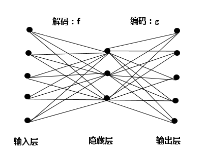
输入层到隐含层的映射关系可以看作是一个编码过程,通过映射函数f把输出向量x映射到隐含层输出y。从隐含层到输出层的过程相当于一个解码过程,把隐含层输出y映射通过映射函数g回去“重构”向量z。对于每一个输入样本x(i)而言,经过自动编码器之后都会转化为一个对应的输出向量z(i)=g[f(x(i))]。当自动编码器训练完成之后,输入X与输出Z完全相同,则对应的隐含层的输出可以看作是输入X的一种抽象表达,因此它可以用于提取输入数据的特征。此外,因为它的隐含层节点数少于输入节点数,因此自动编码器也可以用于降维和数据压缩。网络参数的训练方面,自动编码器采用反向传播法来进行训练,但自动编码器需要大量的训练样本,随着网络结构越变越复杂,网络计算量也随之增大。
对自动编码器结构进行改进得到其他类型的自动编码器,比较典型的是稀疏自动编码器、降噪自动编码器。降噪自动编码器(Denoising Autoencoder,DAE)是对输入数据进行部分“摧毁”,然后通过训练自动编码器模型,重构出原始输入数据,以提高自动编码器的鲁棒性。对输入数据进行“摧毁”的过程其实类似于对数据加入噪声。稀疏自动编码器则是对自动编码器加入一个正则化项,约束隐含层神经元节点大部分输出0,少部分输出非0。稀疏编码器大大减小了需要训练的参数的数目,降低了训练的难度,同时克服了自动编码器容易陷入局部及小值和存在过拟合的问题。降噪编码器采用有噪声的输入数据来训练网络参数,提高了自动编码器的泛化能力。
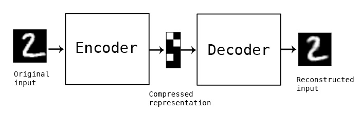
搭建一个自动编码器需要完成下面三样工作:搭建编码器,搭建解码器,设定一个损失函数,用以衡量由于压缩而损失掉的信息。编码器和解码器一般都是参数化的方程,并关于损失函数可导,典型情况是使用神经网络。编码器和解码器的参数可以通过最小化损失函数而优化,例如SGD。
自编码器只是一种思想,在具体实现中,encoder和decoder可以由多种深度学习模型构成,例如全连接层、卷积层或LSTM等,以下使用Keras来实现用于图像去噪的卷积自编码器。
单隐藏层的自编码器
|
|
50个epoch后,看起来自编码器优化的不错了,损失是0.10,我们可视化一下重构出来的输出.上面是原始图像,下面为重构图像,用此方法丢失了太多细节。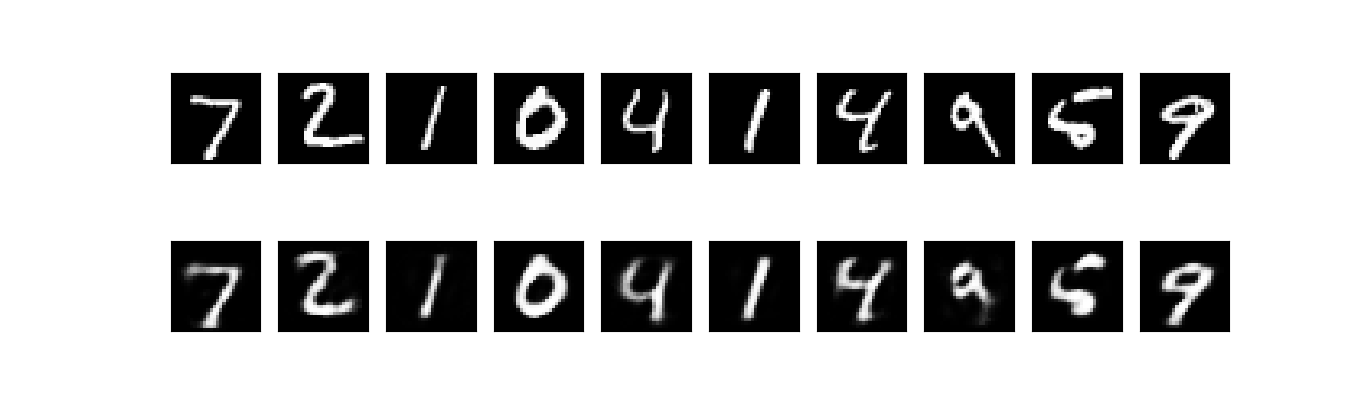
稀疏约束的自编码器
上面的隐层有32个神经元,这种情况下,一般而言自编码器学到的是PCA的一个近似。但是如果我们对隐层单元施加稀疏性约束的话,会得到更为紧凑的表达,只有一小部分神经元会被激活。在Keras中,可以通过添加一个activity_regularizer达到对某层激活值进行约束的目的:
因为添加了正则性约束,所以模型过拟合的风险降低,可以训练多几次,这次训练100个epoch,得到损失为0.11,多出来的0.01基本上是由于正则项造成的。可视化结果如下:
结果上没有什么差别,区别在于编码出来的码字更加稀疏了。稀疏自编码器的在10000个测试图片上的码字均值为3.33,而之前的为7.30
多隐藏层的自编码器
|
|
100个epoch后,loss大概是0.097,比之前的模型好那么一点点。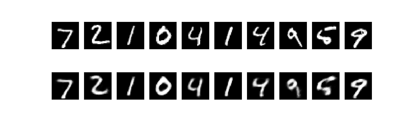
卷积自编码器
由于输入是图像,因此使用卷积神经网络(convnets)作为编码器和解码器是有意义的。在实际设置中,应用于图像的自动编码器始终是卷积自动编码器 - 它们的性能要好得多。编码器将由栈Conv2D和MaxPooling2D层组成(最大池用于空间下采样),而解码器将由Conv2D和UpSampling2D层组成。
自编码器图像去噪
|
|
运行结果:上面一行是添加噪音的图像,下面一行是去噪之后的结果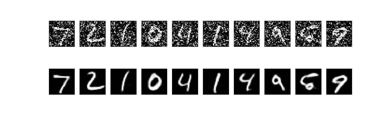
Seq2Seq自编码器
如果输入的是序列,而不是向量或2D图像,首先使用LSTM编码器将输入序列转换成包含整个序列信息的单个向量,然后重复该向量n时间(n输出序列中的时间步长数),并运行一个LSTM解码器将该恒定序列转换成目标序列。
变分自编码 VAE
VAE结构
概率解释的神经网络通过假设每个参数的概率分布来降低网络中每个参数的单个值的刚性约束。例如,在经典神经网络中计算权重w_i=0.7,在概率版本中,计算均值大约为u_i = 0.7和方差为v_i = 0.1的高斯分布,即w_i =N(0.7,0.1)。这个假设将输入,隐藏表示以及神经网络的输出转换为概率随机变量。这类网络被称为贝叶斯神经网络或BNN。
encoder、decoder:均可为任意结构
encoder 又称 recognition model
decoder 又称 generative model
encoder 的输出(2×m 个数)视作分别为 m 个高斯分布的均值(z_mean)和方差的对数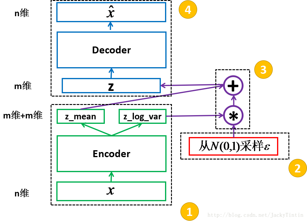
一段VAE伪代码:
采样(sampling)
根据 encoder 输出的均值与方差,生成服从相应高斯分布的随机数:
z 就可以作为上面定义的 decoder 的输入,进而产生 n 维的输出 x^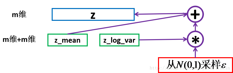
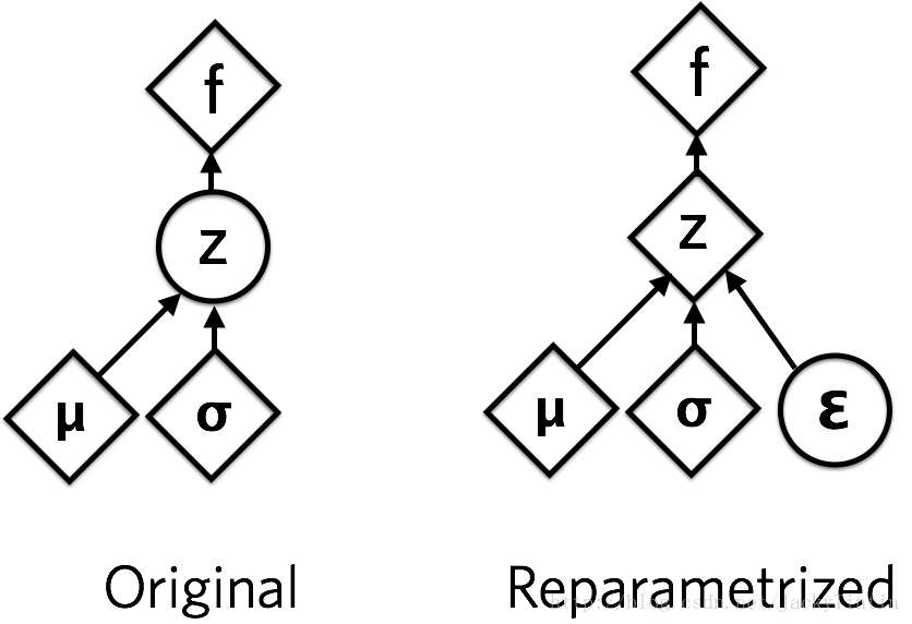
这里运用了 reparemerization 的技巧。由于 z∼N(μ,σ),我们应该从 N(μ,σ) 采样,但这个采样操作对 μ 和 σ 是不可导的,导致常规的通过误差反传的梯度下降法(GD)不能使用。通过 reparemerization,我们首先从 N(0,1) 上采样 ϵ,然后,z=σ⋅ϵ+μ。这样,z∼N(μ,σ),而且,从 encoder 输出到 z,只涉及线性操作,(ϵ 对神经网络而言只是常数),因此,可以正常使用 GD 进行优化。
优化目标
encoder 和 decoder 组合在一起,我们能够对每个 x∈X,输出一个相同维度的 x^。我们目标是,令 x^ 与 x 自身尽量的接近。即 x 经过编码(encode)后,能够通过解码(decode)尽可能多的恢复出原来的信息。
由于 x∈[0,1],因此用交叉熵(cross entropy)度量 x 与 x^ 差异:
$$xent = \sum_{i=1}^n-[x_i\cdot\log(\hat{x}_i)+(1-x_i)\cdot\log(1-\hat{x}_i)]$$
xent 越小,x 与 x^ 越接近。
也可以用均方误差来度量:
$$mse=\sum_{i=1}^n(x_i - \hat{x}_i)^2$$
mse 越小,两者越接近。
另外,需要对 encoder 的输出 z_mean(μ)及 z_log_var(logσ2)加以约束。这里使用的是 KL 散度:
$$KL = -0.5 * (1+\log\sigma^2-\mu^2-\sigma^2)=-0.5(1+\log\sigma^2-\mu^2-exp(\log\sigma^2))$$
总的优化目标(最小化)为:
$$loss = xent + KL$$或者
$$loss = mse + KL$$
综上所述,有了目标函数,并且从输入到输出的所有运算都可导,就可以通过 SGD 或其改进方法来训练这个网络了。训练过程只用到 x(同时作为输入和目标输出),而与 x 的标签无关,因此,这是无监督学习。
代码实现:
VAE形状: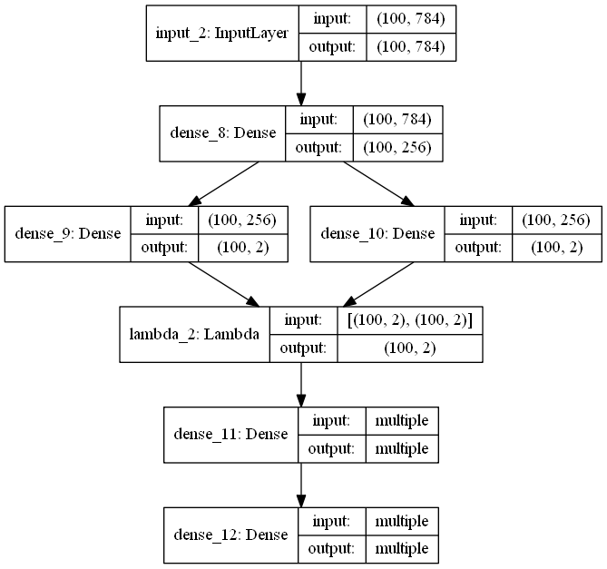
编码器形状: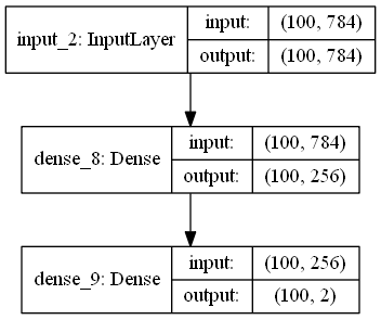
代码中将编码得到的均值U可视化结果: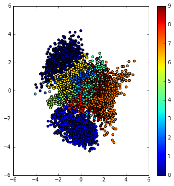
生成器形状: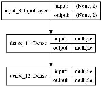
可将从二维高斯分布中随机采样得到的Z,解码成手写数字图片
代码中将解码得到的图像可视化: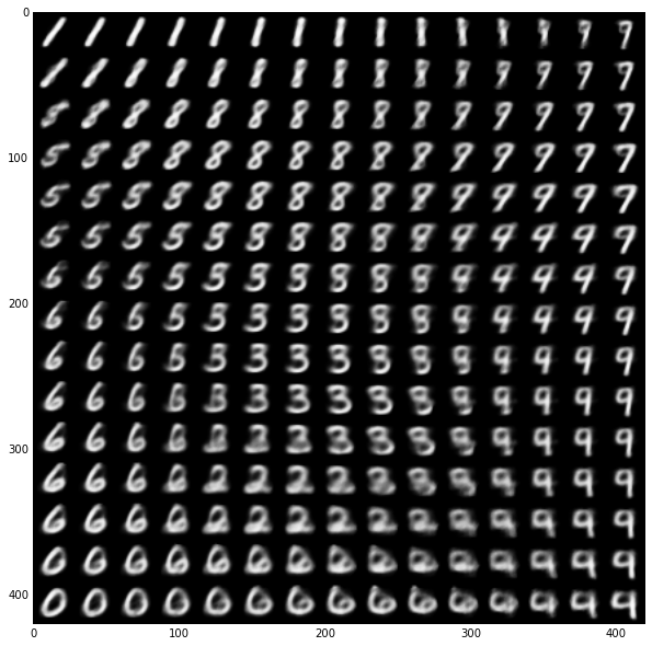
小结
学习算法的最好方式还是读代码,网上有许多基于不同框架的 VAE 参考实现,如
tensorflow 、theano、keras、torch