添加层 def add_layer()
在 Tensorflow 里定义一个添加层的函数可以很容易的添加神经层,为之后的添加省下不少时间.
神经层里常见的参数通常有weights、biases和激励函数。
定义添加神经层的函数 $def add_layer()$ ,它有四个参数:输入值、输入的大小、输出的大小和激励函数,我们设定默认的激励函数是 $None$
接下来定义 $weights$ 和 $biases$
在机器学习中,biases的推荐值不为0,这里是在0向量的基础上又加了0.1。
下面定义Wx_plus_b, 即神经网络未激活的值。其中,tf.matmul()是矩阵的乘法。
当 $activation_function$ ——激励函数为 $None$ 时,输出就是当前的预测值—— $Wx_plus_b$ , 不为 $None$ 时,就把$Wx_plus_b$ 传到 $activation_function()$ 函数中得到输出。
最后,返回输出,添加一个神经层的函数—— $def add_layer()$ 就定义好了。
完整代码:
构造神经网络
构造添加一个神经层的函数。
构建所需的数据。 这里的 $x_data$ 和 $y_data$ 并不是严格的一元二次函数的关系,因为我们多加了一个 $noise$ ,这样看起来会更像真实情况。
利用占位符定义我们所需的神经网络的输入。 $tf.placeholder()$ 就是代表占位符,这里的 $None$ 代表无论输入有多少都可以,因为输入只有一个特征,所以这里是1。
接下来,就可以开始定义神经层了。 通常神经层都包括输入层、隐藏层和输出层。这里的输入层只有一个属性, 所以我们就只有一个输入;隐藏层我们可以自己假设,这里我们假设隐藏层有10个神经元; 输出层和输入层的结构是一样的,所以我们的输出层也是只有一层。 构建的是——输入层1个、隐藏层10个、输出层1个的神经网络。
下面,开始定义隐藏层,利用之前的 $add_layer()$ 函数,这里使用 Tensorflow 自带的激励函数 $tf.nn.relu$.
接着,定义输出层。此时的输入就是隐藏层的输出——l1,输入有10层(隐藏层的输出层),输出有1层.
计算预测值prediction和真实值的误差,对二者差的平方求和再取平均.
接下来,是很关键的一步,如何让机器学习提升它的准确率。$tf.train.GradientDescentOptimizer()$ 中的值通常都小于1,这里取的是0.1,代表以0.1的效率来最小化误差loss.
使用变量时,都要对它进行初始化,这是必不可少的。
定义Session,并用 Session 来执行 init 初始化步骤。 (注意:在tensorflow中,只有 $session.run()$ 才会执行我们定义的运算。)
下面,让机器开始学习。
比如这里让机器学习1000次。机器学习的内容是$train_step$ , 用 $Session$ 来 $run$ 每一次 $training$ 的数据,逐步提升神经网络的预测准确性。 (注意:当运算要用到$placeholder$ 时,就需要 $feed_dict$ 这个字典来指定输入。)
每50步我们输出一下机器学习的误差.
完整代码:
结果可视化
构建图形,用散点图描述真实数据之间的关系。 (注意:plt.ion()用于连续显示。)构建图形,用散点图描述真实数据之间的关系。 (注意:$plt.ion()$ 用于连续显示。)
接下来显示预测数据。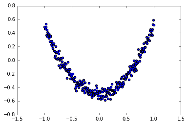
每隔50次训练刷新一次图形,用红色、宽度为5的线来显示我们的预测数据和输入之间的关系,并暂停0.1s。
最后,机器学习的结果为: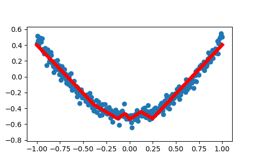
完整代码:
优化器
包括以下几种模式:
●Stochastic Gradient Descent (SGD)
●Momentum
●AdaGrad
●RMSProp
●Adam
越复杂的神经网络 , 越多的数据 , 需要在训练神经网络的过程上花费的时间也就越多. 原因很简单, 就是因为计算量太大了. 可是往往有时候为了解决复杂的问题, 复杂的结构和大数据又是不能避免的, 所以我们需要寻找一些方法, 让神经网络聪明起来, 快起来.
Stochastic Gradient Descent (SGD)
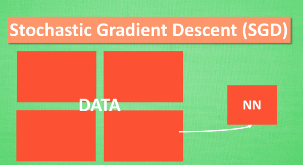
所以, 最基础的方法就是 SGD 啦, 想像红色方块是我们要训练的 data, 如果用普通的训练方法, 就需要重复不断的把整套数据放入神经网络 NN训练, 这样消耗的计算资源会很大.
换一种思路, 如果把这些数据拆分成小批小批的, 然后再分批不断放入 NN 中计算, 这就是常说的 SGD 的正确打开方式了. 每次使用批数据, 虽然不能反映整体数据的情况, 不过却很大程度上加速了 NN 的训练过程, 而且也不会丢失太多准确率.如果运用上了 SGD, 你还是嫌训练速度慢, 那怎么办?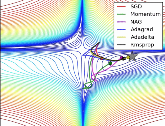
没问题, 事实证明, SGD 并不是最快速的训练方法, 红色的线是 SGD, 但它到达学习目标的时间是在这些方法中最长的一种. 我们还有很多其他的途径来加速训练.
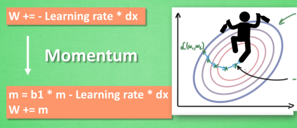
Momentum 更新方法
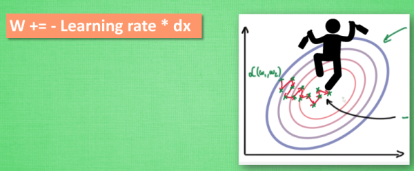
大多数其他途径是在更新神经网络参数那一步上动动手脚. 传统的参数 W 的更新是把原始的 W 累加上一个负的学习率(learning rate) 乘以校正值 (dx). 这种方法可能会让学习过程曲折无比, 看起来像 喝醉的人回家时, 摇摇晃晃走了很多弯路.
所以我们把这个人从平地上放到了一个斜坡上, 只要他往下坡的方向走一点点, 由于向下的惯性, 他不自觉地就一直往下走, 走的弯路也变少了. 这就是 Momentum 参数更新. 另外一种加速方法叫AdaGrad.
AdaGrad 更新方法
这种方法是在学习率上面动手脚, 使得每一个参数更新都会有自己与众不同的学习率, 他的作用和 momentum 类似, 不过不是给喝醉酒的人安排另一个下坡, 而是给他一双不好走路的鞋子, 使得他一摇晃着走路就脚疼, 鞋子成为了走弯路的阻力, 逼着他往前直着走. 他的数学形式是这样的. 接下来又有什么方法呢? 如果把下坡和不好走路的鞋子合并起来, 是不是更好呢? 没错, 这样我们就有了 RMSProp 更新方法.
RMSProp 更新方法
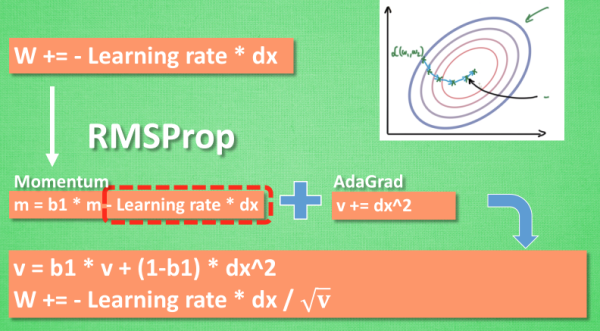
有了 momentum 的惯性原则 , 加上 adagrad 的对错误方向的阻力, 我们就能合并成这样. 让 RMSProp同时具备他们两种方法的优势. 不过细心的同学们肯定看出来了, 似乎在 RMSProp 中少了些什么. 原来是我们还没把 Momentum合并完全, RMSProp 还缺少了 momentum 中的 这一部分. 所以, 我们在 Adam 方法中补上了这种想法.
Adam 更新方法
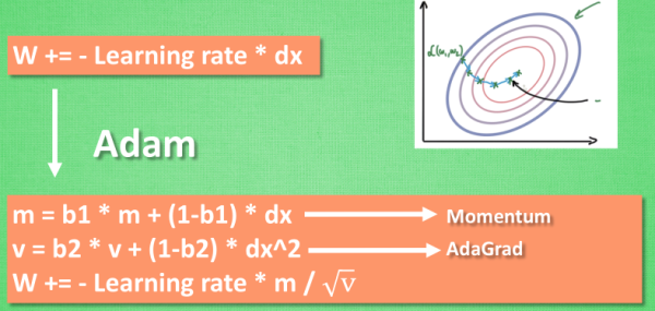
计算m 时有 momentum 下坡的属性, 计算 v 时有 adagrad 阻力的属性, 然后再更新参数时 把 m 和 V 都考虑进去. 实验证明, 大多数时候, 使用 adam 都能又快又好的达到目标, 迅速收敛. 所以说, 在加速神经网络训练的时候, 一个下坡, 一双破鞋子, 功不可没.