Keras下可视化神经网络

windows 10 & Python 3.5
1.下载graphviz-2.3.8.msi并安装,官网:http://www.graphviz.org/Download_windows.php
添加环境变量:C:\Program Files (x86)\Graphviz2.38\bin
2.pip install graphviz (0.7)
3.pip install pydot (1.2.3)

1
2
3
4
5
6
7
8
9
10
11
12
13
14
15
16
17
18
19
20
21
22
23
24
import numpy as np
from keras.models import Sequential
from keras.layers.core import Dense, Activation
from keras.optimizers import SGD
from keras.utils import np_utils
from keras.utils import plot_model
# keras 1.0 use:
# from keras.utils.visualize_util import plot
def run():
# 构建神经网络
model = Sequential()
model.add(Dense(4, input_dim=2, init='uniform'))
model.add(Activation('relu'))
model.add(Dense(2, init='uniform'))
model.add(Activation('sigmoid'))
sgd = SGD(lr=0.05, decay=1e-6, momentum=0.9, nesterov=True)
model.compile(loss='binary_crossentropy', optimizer=sgd, metrics=['accuracy'])
# 神经网络可视化
plot_model(model, to_file='model.png')
if __name__ == '__main__':
run()

可视化结果:
img

Ubuntu 16.04 & Python 2.7
1.sudo pip install graphviz (0.7)
2.sudo apt-get install graphviz (2.38.0-16)
3.sudo pip install pydot==1.1.0 (1.2.3的版本find_graphviz函数会报错)
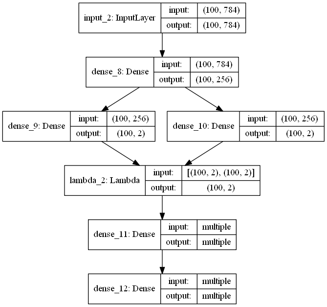
来个VAE网络试试:

1
2
3
4
5
6
7
8
9
10
11
12
13
14
15
16
17
18
19
20
21
22
23
24
25
26
27
28
29
30
31
32
33
34
35
36
37
38
39
40
41
42
43
44
45
46
47
48
49
50
51
52
53
54
55
56
57
58
59
60
61
62
63
64
65
66
67
68
69
70
71
72
73
74
75
76
77
78
79
80
81
82
83
84
85
86
87
88
89
90
91
92
93
94
95
96
97
98
99
100
101
102
103
104
105
106
107
108
109
110
111
112
113
114
115
116
117
118
119
# -*- coding: utf-8 -*-
’‘’
Reference: "Auto-Encoding Variational Bayes" https://arxiv.org/abs/1312.6114
‘’‘
import numpy as np
import matplotlib.pyplot as plt
from scipy.stats import norm
from keras.layers import Input, Dense, Lambda
from keras.models import Model
from keras import backend as K
from keras import objectives
from keras.datasets import mnist
from keras.utils import plot_model
import sys
saveout = sys.stdout
file = open('variational_autoencoder.txt','w')
sys.stdout = file
batch_size = 100
original_dim = 784 #28*28
latent_dim = 2
intermediate_dim = 256
nb_epoch = 50
epsilon_std = 1.0
#my tips:encoding
x = Input(batch_shape=(batch_size, original_dim))
h = Dense(intermediate_dim, activation='relu')(x)
z_mean = Dense(latent_dim)(h)
z_log_var = Dense(latent_dim)(h)
#my tips:Gauss sampling,sample Z
def sampling(args):
z_mean, z_log_var = args
epsilon = K.random_normal(shape=(batch_size, latent_dim), mean=0.,
stddev=epsilon_std)
return z_mean + K.exp(z_log_var / 2) * epsilon
# note that "output_shape" isn't necessary with the TensorFlow backend
# my tips:get sample z(encoded)
z = Lambda(sampling, output_shape=(latent_dim,))([z_mean, z_log_var])
# we instantiate these layers separately so as to reuse them later
decoder_h = Dense(intermediate_dim, activation='relu')
decoder_mean = Dense(original_dim, activation='sigmoid')
h_decoded = decoder_h(z)
x_decoded_mean = decoder_mean(h_decoded)
#my tips:loss(restruct X)+KL
def vae_loss(x, x_decoded_mean):
#my tips:logloss
xent_loss = original_dim * objectives.binary_crossentropy(x, x_decoded_mean)
#my tips:see paper's appendix B
kl_loss = - 0.5 * K.sum(1 + z_log_var - K.square(z_mean) - K.exp(z_log_var), axis=-1)
return xent_loss + kl_loss
vae = Model(x, x_decoded_mean)
vae.compile(optimizer='rmsprop', loss=vae_loss)
# train the VAE on MNIST digits
(x_train, y_train), (x_test, y_test) = mnist.load_data(path='mnist.pkl.gz')
x_train = x_train.astype('float32') / 255.
x_test = x_test.astype('float32') / 255.
x_train = x_train.reshape((len(x_train), np.prod(x_train.shape[1:])))
x_test = x_test.reshape((len(x_test), np.prod(x_test.shape[1:])))
vae.fit(x_train, x_train,
shuffle=True,
nb_epoch=nb_epoch,
verbose=2,
batch_size=batch_size,
validation_data=(x_test, x_test))
# build a model to project inputs on the latent space
encoder = Model(x, z_mean)
# display a 2D plot of the digit classes in the latent space
x_test_encoded = encoder.predict(x_test, batch_size=batch_size)
plt.figure(figsize=(6, 6))
plt.scatter(x_test_encoded[:, 0], x_test_encoded[:, 1], c=y_test)
plt.colorbar()
plt.show()
# build a digit generator that can sample from the learned distribution
decoder_input = Input(shape=(latent_dim,))
_h_decoded = decoder_h(decoder_input)
_x_decoded_mean = decoder_mean(_h_decoded)
generator = Model(decoder_input, _x_decoded_mean)
# display a 2D manifold of the digits
n = 15 # figure with 15x15 digits
digit_size = 28
figure = np.zeros((digit_size * n, digit_size * n))
# linearly spaced coordinates on the unit square were transformed through the inverse CDF (ppf) of the Gaussian
# to produce values of the latent variables z, since the prior of the latent space is Gaussian
grid_x = norm.ppf(np.linspace(0.05, 0.95, n))
grid_y = norm.ppf(np.linspace(0.05, 0.95, n))
for i, yi in enumerate(grid_x):
for j, xi in enumerate(grid_y):
z_sample = np.array([[xi, yi]])
x_decoded = generator.predict(z_sample)
digit = x_decoded[0].reshape(digit_size, digit_size)
figure[i * digit_size: (i + 1) * digit_size,
j * digit_size: (j + 1) * digit_size] = digit
plt.figure(figsize=(10, 10))
plt.imshow(figure, cmap='Greys_r')
plt.show()
plot_model(vae,to_file='variational_autoencoder_vae.png',show_shapes=True)
plot_model(encoder,to_file='variational_autoencoder_encoder.png',show_shapes=True)
plot_model(generator,to_file='variational_autoencoder_generator.png',show_shapes=True)
sys.stdout.close()
sys.stdout = saveout

可视化结果:
img

如果文章对您有用请随意打赏,谢谢支持!
0%