相关背景资料
主题模型采用LSI(Latent semantic indexing, 中文译为浅层语义索引),LSI区别LSA(Latent semantic analysis,中文译为浅层语义分析)
1) TF-IDF,余弦相似度,向量空间模型
TF-IDF与余弦相似性的应用(一):自动提取关键词、TF-IDF与余弦相似性的应用(二):找出相似文章
2)SVD和LSI
想了解LSI一定要知道SVD(Singular value decomposition, 中文译为奇异值分解),而SVD的作用不仅仅局限于LSI,在很多地方都能见到其身影,SVD自诞生之后,其应用领域不断被发掘,可以不夸张的说如果学了线性代数而不明白SVD,基本上等于没学。教程:机器学习中的数学(4)-线性判别分析(LDA), 主成分分析(PCA)、机器学习中的数学(5)-强大的矩阵奇异值分解(SVD)及其应用
关于LSI,简单说两句,一种情况下考察两个词的关系常常考虑的是它们在一个窗口长度(譬如一句话,一段话或一个文章)里的共现情况,在语料库语言学里有个专业点叫法叫Collocation,中文译为搭配或词语搭配。而LSI所做的是挖掘如下这层词语关系:A和C共现,B和C共现,目标是找到A和B的隐含关系,学术一点的叫法是second-order co-ocurrence。以下引用百度空间上一篇介绍相关参考资料时的简要描述:
LSI本质上识别了以文档为单位的second-order co-ocurrence的单词并归入同一个子空间。因此:
1)落在同一子空间的单词不一定是同义词,甚至不一定是在同情景下出现的单词,对于长篇文档尤其如是。
2)LSI根本无法处理一词多义的单词(多义词),多义词会导致LSI效果变差。
A persistent myth in search marketing circles is that LSI grants contextuality; i.e., terms occurring in the same context. This is not always the case. Consider two documents X and Y and three terms A, B and C and wherein:
A and B do not co-occur.
X mentions terms A and C
Y mentions terms B and C.
:. A—C—B
The common denominator is C, so we define this relation as an in-transit co-occurrence since both A and B occur while in transit with C. This is called second-order co-occurrence and is a special case of high-order co-occurrence.
PDF Tutorial版本:
Singular Value Decomposition (SVD)- A Fast Track Tutorial
Latent Semantic Indexing (LSI) A Fast Track Tutorial
3) LDA
机器学习中的数学(4)-线性判别分析(LDA), 主成分分析(PCA)
gensim基本使用
from gensim import corpora, models, similarities
import logging
logging.basicConfig(format='%(asctime)s : %(levelname)s : %(message)s', level=logging.INFO)
然后将上面那个文档中的例子作为文档输入,在Python中用document list表示:
documents = ["Shipment of gold damaged in a fire",
"Delivery of silver arrived in a silver truck",
"Shipment of gold arrived in a truck"]
正常情况下,需要对英文文本做一些预处理工作,譬如去停用词,对文本进行tokenize,stemming以及过滤掉低频的词,但是为了说明问题,也是为了和这篇”LSI Fast Track Tutorial”保持一致,以下的预处理仅仅是将英文单词小写化:
texts = [[word for word in document.lower().split()] for document in documents]
print texts
#[['shipment', 'of', 'gold', 'damaged', 'in', 'a', 'fire'], ['delivery', 'of', 'silver', 'arrived', 'in', 'a', 'silver', 'truck'], ['shipment', 'of', 'gold', 'arrived', 'in', 'a', 'truck']]
我们可以通过这些文档抽取一个“词袋(bag-of-words)”,将文档的token映射为id:
dictionary = corpora.Dictionary(texts)
print dictionary
#Dictionary(11 unique tokens)
print dictionary.token2id
#{'a': 0, 'damaged': 1, 'gold': 3, 'fire': 2, 'of': 5, 'delivery': 8, 'arrived': 7, 'shipment': 6, 'in': 4, 'truck': 10, 'silver': 9}
然后就可以将用字符串表示的文档转换为用id表示的文档向量:
corpus = [dictionary.doc2bow(text) for text in texts]
print corpus
#[[(0, 1), (1, 1), (2, 1), (3, 1), (4, 1), (5, 1), (6, 1)], [(0, 1), (4, 1), (5, 1), (7, 1), (8, 1), (9, 2), (10, 1)], [(0, 1), (3, 1), (4, 1), (5, 1), (6, 1), (7, 1), (10, 1)]]
例如(9,2)这个元素代表第二篇文档中id为9的单词“silver”出现了2次。
有了这些信息,我们就可以基于这些“训练文档”计算一个TF-IDF“模型”:
tfidf = models.TfidfModel(corpus)
基于这个TF-IDF模型,我们可以将上述用词频表示文档向量表示为一个用tf-idf值表示的文档向量:
corpus_tfidf = tfidf[corpus]
for doc in corpus_tfidf:
... print doc
#[(1, 0.6633689723434505), (2, 0.6633689723434505), (3, 0.2448297500958463), (6, 0.2448297500958463)]
[(7, 0.16073253746956623), (8, 0.4355066251613605), (9, 0.871013250322721), (10, 0.16073253746956623)]
[(3, 0.5), (6, 0.5), (7, 0.5), (10, 0.5)]
发现一些token貌似丢失了,我们打印一下tfidf模型中的信息:
print tfidf.dfs
#{0: 3, 1: 1, 2: 1, 3: 2, 4: 3, 5: 3, 6: 2, 7: 2, 8: 1, 9: 1, 10: 2}
print tfidf.idfs
#{0: 0.0, 1: 1.5849625007211563, 2: 1.5849625007211563, 3: 0.5849625007211562, 4: 0.0, 5: 0.0, 6: 0.5849625007211562, 7: 0.5849625007211562, 8: 1.5849625007211563, 9: 1.5849625007211563, 10: 0.5849625007211562}
我们发现由于包含id为0, 4, 5这3个单词的文档数(df)为3,而文档总数也为3,所以idf被计算为0了,看来gensim没有对分子加1,做一个平滑。不过我们同时也发现这3个单词分别为a, in, of这样的介词,完全可以在预处理时作为停用词干掉,这也从另一个方面说明TF-IDF的有效性。
有了tf-idf值表示的文档向量,我们就可以训练一个LSI模型,和Latent Semantic Indexing (LSI) A Fast Track Tutorial中的例子相似,我们设置topic数为2:
lsi = models.LsiModel(corpus_tfidf, id2word=dictionary, num_topics=2)
lsi.print_topics(2)
# topic #0(1.137): 0.438*"gold" + 0.438*"shipment" + 0.366*"truck" + 0.366*"arrived" + 0.345*"damaged" + 0.345*"fire" + 0.297*"silver" + 0.149*"delivery" + 0.000*"in" + 0.000*"a"
topic #1(1.000): 0.728*"silver" + 0.364*"delivery" + -0.364*"fire" + -0.364*"damaged" + 0.134*"truck" + 0.134*"arrived" + -0.134*"shipment" + -0.134*"gold" + -0.000*"a" + -0.000*"in"
lsi的物理意义不太好解释,不过最核心的意义是将训练文档向量组成的矩阵SVD分解,并做了一个秩为2的近似SVD分解,可以参考那篇英文tutorail。有了这个lsi模型,我们就可以将文档映射到一个二维的topic空间中:
corpus_lsi = lsi[corpus_tfidf]
for doc in corpus_lsi:
... print doc
#[(0, 0.67211468809878649), (1, -0.54880682119355917)]
[(0, 0.44124825208697727), (1, 0.83594920480339041)]
[(0, 0.80401378963792647)]
可以看出,文档1,3和topic1更相关,文档2和topic2更相关;
我们也可以顺手跑一个LDA模型:
lda = models.LdaModel(copurs_tfidf, id2word=dictionary, num_topics=2)
lda.print_topics(2)
#topic #0: 0.119*silver + 0.107*shipment + 0.104*truck + 0.103*gold + 0.102*fire + 0.101*arrived + 0.097*damaged + 0.085*delivery + 0.061*of + 0.061*in
topic #1: 0.110*gold + 0.109*silver + 0.105*shipment + 0.105*damaged + 0.101*arrived + 0.101*fire + 0.098*truck + 0.090*delivery + 0.061*of + 0.061*in
lda模型中的每个主题单词都有概率意义,其加和为1,值越大权重越大,物理意义比较明确,不过反过来再看这三篇文档训练的2个主题的LDA模型太平均了,没有说服力。
好了,我们回到LSI模型,有了LSI模型,我们如何来计算文档直接的相思度,或者换个角度,给定一个查询Query,如何找到最相关的文档?当然首先是建索引了:
index = similarities.MatrixSimilarity(lsi[corpus])
还是以这篇英文tutorial中的查询Query为例:gold silver truck。首先将其向量化:
query = "gold silver truck"
query_bow = dictionary.doc2bow(query.lower().split())
print query_bow
[(3, 1), (9, 1), (10, 1)]
再用之前训练好的LSI模型将其映射到二维的topic空间:
query_lsi = lsi[query_bow]
print query_lsi
[(0, 1.1012835748628467), (1, 0.72812283398049593)]
最后就是计算其和index中doc的余弦相似度了:
sims = index[query_lsi]
print list(enumerate(sims))
[(0, 0.40757114), (1, 0.93163693), (2, 0.83416492)]
当然,我们也可以按相似度进行排序:
sort_sims = sorted(enumerate(sims), key=lambda item: -item[1])
print sort_sims
[(1, 0.93163693), (2, 0.83416492), (0, 0.40757114)]
可以看出,这个查询的结果是doc2 > doc3 > doc1,和fast tutorial是一致的,虽然数值上有一些差别: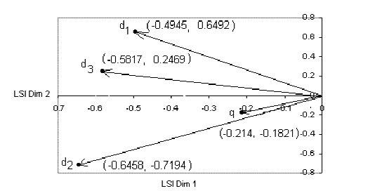
计算两个文档的相似度
本节将主要说明如何基于gensim计算课程图谱上课程之间的主题相似度,同时考虑一些改进方法,包括借助英文的自然语言处理工具包NLTK以及用更大的维基百科的语料来看看效果。
1、数据准备
这里准备了一份Coursera的课程数据,可以在这里下载:coursera_corpus,(百度网盘链接: http://t.cn/RhjgPkv, 密码: oppc)总共379个课程,每行包括3部分内容:课程名\t课程简介\t课程详情, 已经清除了其中的html tag, 下面所示的例子仅仅是其中的课程名:
Writing II: Rhetorical Composing
Genetics and Society: A Course for Educators
General Game Playing
Genes and the Human Condition (From Behavior to Biotechnology)
A Brief History of Humankind
New Models of Business in Society
Analyse Numérique pour Ingénieurs
Evolution: A Course for Educators
Coding the Matrix: Linear Algebra through Computer Science Applications
The Dynamic Earth: A Course for Educators
...
首先加载数据:
from gensim import corpora, models, similarities
import logging
logging.basicConfig(format='%(asctime)s : %(levelname)s : %(message)s', level=logging.INFO)
import csv

file = open("coursera_corpus",'r',encoding = 'UTF8')
courses = [line.strip() for line in file]
courses_name = [course.split('\t')[0] for course in courses]
print(courses_name[0:10])

#['Writing II: Rhetorical Composing', 'Genetics and Society: A Course for Educators', 'General Game Playing', 'Genes and the Human Condition (From Behavior to Biotechnology)', 'A Brief History of Humankind', 'New Models of Business in Society', 'Analyse Num\xc3\xa9rique pour Ing\xc3\xa9nieurs', 'Evolution: A Course for Educators', 'Coding the Matrix: Linear Algebra through Computer Science Applications', 'The Dynamic Earth: A Course for Educators']
2、引入NLTK
NTLK是著名的Python自然语言处理工具包,但是主要针对的是英文处理,不过课程图谱目前处理的课程数据主要是英文,因此也足够了。
import nltk
nltk.download()
现在来处理刚才的课程数据,如果按此前的方法仅仅对文档的单词小写化的话,将得到如下的结果:
exts_lower = [[word for word in document.lower().split()] for document in courses]
print texts_lower[0]
#['writing', 'ii:', 'rhetorical', 'composing', 'rhetorical', 'composing', 'engages', 'you', 'in', 'a', 'series', 'of', 'interactive', 'reading,', 'research,', 'and', 'composing', 'activities', 'along', 'with', 'assignments', 'designed', 'to', 'help', 'you', 'become', 'more', 'effective', 'consumers', 'and', 'producers', 'of', 'alphabetic,', 'visual', 'and', 'multimodal', 'texts.', 'join', 'us', 'to', 'become', 'more', 'effective', 'writers...', 'and', 'better', 'citizens.', 'rhetorical', 'composing', 'is', 'a', 'course', 'where', 'writers', 'exchange', 'words,', 'ideas,', 'talents,', 'and', 'support.', 'you', 'will', 'be', 'introduced', 'to', 'a', ...
注意其中很多标点符号和单词是没有分离的,所以我们引入nltk的word_tokenize函数,并处理相应的数据:
from nltk.tokenize import word_tokenize
texts_tokenized = [[word.lower() for word in word_tokenize(document.decode('utf-8'))] for document in courses]
print texts_tokenized[0]
#['writing', 'ii', ':', 'rhetorical', 'composing', 'rhetorical', 'composing', 'engages', 'you', 'in', 'a', 'series', 'of', 'interactive', 'reading', ',', 'research', ',', 'and', 'composing', 'activities', 'along', 'with', 'assignments', 'designed', 'to', 'help', 'you', 'become', 'more', 'effective', 'consumers', 'and', 'producers', 'of', 'alphabetic', ',', 'visual', 'and', 'multimodal', 'texts.', 'join', 'us', 'to', 'become', 'more', 'effective', 'writers', '...', 'and', 'better', 'citizens.', 'rhetorical', 'composing', 'is', 'a', 'course', 'where', 'writers', 'exchange', 'words', ',', 'ideas', ',', 'talents', ',', 'and', 'support.', 'you', 'will', 'be', 'introduced', 'to', 'a', ...
对课程的英文数据进行tokenize之后,我们需要去停用词,幸好NLTK提供了一份英文停用词数据:
from nltk.corpus import stopwords
english_stopwords = stopwords.words('english')
print english_stopwords
#['i', 'me', 'my', 'myself', 'we', 'our', 'ours', 'ourselves', 'you', 'your', 'yours', 'yourself', 'yourselves', 'he', 'him', 'his', 'himself', 'she', 'her', 'hers', 'herself', 'it', 'its', 'itself', 'they', 'them', 'their', 'theirs', 'themselves', 'what', 'which', 'who', 'whom', 'this', 'that', 'these', 'those', 'am', 'is', 'are', 'was', 'were', 'be', 'been', 'being', 'have', 'has', 'had', 'having', 'do', 'does', 'did', 'doing', 'a', 'an', 'the', 'and', 'but', 'if', 'or', 'because', 'as', 'until', 'while', 'of', 'at', 'by', 'for', 'with', 'about', 'against', 'between', 'into', 'through', 'during', 'before', 'after', 'above', 'below', 'to', 'from', 'up', 'down', 'in', 'out', 'on', 'off', 'over', 'under', 'again', 'further', 'then', 'once', 'here', 'there', 'when', 'where', 'why', 'how', 'all', 'any', 'both', 'each', 'few', 'more', 'most', 'other', 'some', 'such', 'no', 'nor', 'not', 'only', 'own', 'same', 'so', 'than', 'too', 'very', 's', 't', 'can', 'will', 'just', 'don', 'should', 'now']
len(english_stopwords)
#127
总计127个停用词,我们首先过滤课程语料中的停用词:
texts_filtered_stopwords = [[word for word in document if not word in english_stopwords] for document in texts_tokenized]
print texts_filtered_stopwords[0]
#['writing', 'ii', ':', 'rhetorical', 'composing', 'rhetorical', 'composing', 'engages', 'series', 'interactive', 'reading', ',', 'research', ',', 'composing', 'activities', 'along', 'assignments', 'designed', 'help', 'become', 'effective', 'consumers', 'producers', 'alphabetic', ',', 'visual', 'multimodal', 'texts.', 'join', 'us', 'become', 'effective', 'writers', '...', 'better', 'citizens.', 'rhetorical', 'composing', 'course', 'writers', 'exchange', 'words', ',', 'ideas', ',', 'talents', ',', 'support.', 'introduced', 'variety', 'rhetorical', 'concepts\xe2\x80\x94that', ',', 'ideas', 'techniques', 'inform', 'persuade', 'audiences\xe2\x80\x94that', 'help', 'become', 'effective', 'consumer', 'producer', 'written', ',', 'visual', ',', 'multimodal', 'texts.', 'class', 'includes', 'short', 'videos', ',', 'demonstrations', ',', 'activities.', 'envision', 'rhetorical', 'composing', 'learning', 'community', 'includes', 'enrolled', 'course', 'instructors.', 'bring', 'expertise', 'writing', ',', 'rhetoric', 'course', 'design', ',', 'designed', 'assignments', 'course', 'infrastructure', 'help', 'share', 'experiences', 'writers', ',', 'students', ',', 'professionals', 'us.', 'collaborations', 'facilitated', 'wex', ',', 'writers', 'exchange', ',', 'place', 'exchange', 'work', 'feedback']
停用词被过滤了,不过发现标点符号还在,这个好办,我们首先定义一个标点符号list:
english_punctuations = [',', '.', ':', ';', '?', '(', ')', '[', ']', '&', '!', '*', '@', '#', '$', '%']

然后过滤这些标点符号:

texts_filtered = [[word for word in document if not word in english_punctuations] for document in texts_filtered_stopwords]
print texts_filtered[0]
#['writing', 'ii', 'rhetorical', 'composing', 'rhetorical', 'composing', 'engages', 'series', 'interactive', 'reading', 'research', 'composing', 'activities', 'along', 'assignments', 'designed', 'help', 'become', 'effective', 'consumers', 'producers', 'alphabetic', 'visual', 'multimodal', 'texts.', 'join', 'us', 'become', 'effective', 'writers', '...', 'better', 'citizens.', 'rhetorical', 'composing', 'course', 'writers', 'exchange', 'words', 'ideas', 'talents', 'support.', 'introduced', 'variety', 'rhetorical', 'concepts\xe2\x80\x94that', 'ideas', 'techniques', 'inform', 'persuade', 'audiences\xe2\x80\x94that', 'help', 'become', 'effective', 'consumer', 'producer', 'written', 'visual', 'multimodal', 'texts.', 'class', 'includes', 'short', 'videos', 'demonstrations', 'activities.', 'envision', 'rhetorical', 'composing', 'learning', 'community', 'includes', 'enrolled', 'course', 'instructors.', 'bring', 'expertise', 'writing', 'rhetoric', 'course', 'design', 'designed', 'assignments', 'course', 'infrastructure', 'help', 'share', 'experiences', 'writers', 'students', 'professionals', 'us.', 'collaborations', 'facilitated', 'wex', 'writers', 'exchange', 'place', 'exchange', 'work', 'feedback']
更进一步,我们对这些英文单词词干化(Stemming),NLTK提供了好几个相关工具接口可供选择,具体参考这个页面: http://nltk.org/api/nltk.stem.html , 可选的工具包括Lancaster Stemmer, Porter Stemmer等知名的英文Stemmer。这里我们使用LancasterStemmer:
from nltk.stem.lancaster import LancasterStemmer
st = LancasterStemmer()
st.stem('stemmed')
#'stem'
st.stem('stemming')
#'stem'
st.stem('stemmer')
#'stem'
st.stem('running')
#'run'
st.stem('maximum')
#'maxim'
st.stem('presumably')
#'presum'
让我们调用这个接口来处理上面的课程数据:
texts_stemmed = [[st.stem(word) for word in docment] for docment in texts_filtered]
print texts_stemmed[0]
#['writ', 'ii', 'rhet', 'compos', 'rhet', 'compos', 'eng', 'sery', 'interact', 'read', 'research', 'compos', 'act', 'along', 'assign', 'design', 'help', 'becom', 'effect', 'consum', 'produc', 'alphabet', 'vis', 'multimod', 'texts.', 'join', 'us', 'becom', 'effect', 'writ', '...', 'bet', 'citizens.', 'rhet', 'compos', 'cours', 'writ', 'exchang', 'word', 'idea', 'tal', 'support.', 'introduc', 'vary', 'rhet', 'concepts\xe2\x80\x94that', 'idea', 'techn', 'inform', 'persuad', 'audiences\xe2\x80\x94that', 'help', 'becom', 'effect', 'consum', 'produc', 'writ', 'vis', 'multimod', 'texts.', 'class', 'includ', 'short', 'video', 'demonst', 'activities.', 'envid', 'rhet', 'compos', 'learn', 'commun', 'includ', 'enrol', 'cours', 'instructors.', 'bring', 'expert', 'writ', 'rhet', 'cours', 'design', 'design', 'assign', 'cours', 'infrastruct', 'help', 'shar', 'expery', 'writ', 'stud', 'profess', 'us.', 'collab', 'facilit', 'wex', 'writ', 'exchang', 'plac', 'exchang', 'work', 'feedback']
在我们引入gensim之前,还有一件事要做,去掉在整个语料库中出现次数为1的低频词,测试了一下,不去掉的话对效果有些影响:
all_stems = sum(texts_stemmed, [])
stems_once = set(stem for stem in set(all_stems) if all_stems.count(stem) ==
texts = [[stem for stem in text if stem not in stems_once] for text in texts_stemmed]
3、引入gensim
有了上述的预处理,我们就可以引入gensim,并快速的做课程相似度的实验了。以下会快速的过一遍流程,具体的可以参考上一节的详细描述。
from gensim import corpora, models, similarities
import logging
logging.basicConfig(format='%(asctime)s : %(levelname)s : %(message)s', level=logging.INFO)

dictionary = corpora.Dictionary(texts)
corpus = [dictionary.doc2bow(text) for text in texts]
tfidf = models.TfidfModel(corpus)
corpus_tfidf = tfidf[corpus]
#这里我训练topic数量为10的LSI模型:
lsi = models.LsiModel(corpus_tfidf, id2word=dictionary, num_topics=10)

index = similarities.MatrixSimilarity(lsi[corpus])
基于LSI模型的课程索引建立完毕,我们以Andrew Ng教授的机器学习公开课为例,这门课程在我们的coursera_corpus文件的第211行,也就是:
 print courses_name[210]
#Machine Learning
现在我们就可以通过lsi模型将这门课程映射到10个topic主题模型空间上,然后和其他课程计算相似度:
ml_course = texts[210]
ml_bow = dicionary.doc2bow(ml_course)
ml_lsi = lsi[ml_bow]
print ml_lsi
#[(0, 8.3270084238788673), (1, 0.91295652151975082), (2, -0.28296075112669405), (3, 0.0011599008827843801), (4, -4.1820134980024255), (5, -0.37889856481054851), (6, 2.0446999575052125), (7, 2.3297944485200031), (8, -0.32875594265388536), (9, -0.30389668455507612)]

sims = index[ml_lsi]
sort_sims = sorted(enumerate(sims), key=lambda item: -item[1])


取按相似度排序的前10门课程:
print sort_sims[0:10]
#[(210, 1.0), (174, 0.97812241), (238, 0.96428639), (203, 0.96283489), (63, 0.9605484), (189, 0.95390636), (141, 0.94975704), (184, 0.94269753), (111, 0.93654782), (236, 0.93601125)]

第一门课程是它自己:
print courses_name[210]
#Machine Learning

第二门课是Coursera上另一位大牛Pedro Domingos机器学习公开课
print courses_name[174]
#Machine Learning

第三门课是Coursera的另一位创始人,同样是大牛的Daphne Koller教授的概率图模型公开课:
print courses_name[238]
#Probabilistic Graphical Models

第四门课是另一位超级大牛Geoffrey Hinton的神经网络公开课,有同学评价是Deep Learning的必修课。
print courses_name[203]
#Neural Networks for Machine Learning